Exploring OpenStreetMap with Rust

In this post, we will explore OpenStreetMap, an open geospatial dataset, using Rust.

Background

The reason we focused on Rust is that we increasingly need higher-resolution solutions for large and complex transportation data problems. At NearMe, most of our system is currently written in TypeScript, while parts related to optimization algorithms are written in Python. This setup worked well in our startup phase, but as we pursue further tuning, Rust became a promising option.

Rust offers C/C++-class performance, safe and efficient memory management, and many features that improve developer productivity. In Python, you can still combine performance and productivity by implementing low-level routines in C/C++ and writing high-level logic in Python, but depending on the problem, that approach has limits. On the other hand, writing everything in C/C++ is also costly. Rust may not be as concise as Python, but compared to C++, it can deliver speed and safety with less effort. A deeper comparison with languages like Go would take more space, but in short, we considered Rust because it is closer to the role C++ often plays in algorithm-heavy systems.

Also, because NearMe is built with a microservices architecture, we can choose either to write low-level components in Rust and bind them, or to build an entire microservice in Rust. Of course, adding another language has trade-offs, so we need to evaluate carefully. Even so, Rust stands out as a unique and promising candidate.

As a first step in learning Rust, we will load and visualize OpenStreetMap data. OpenStreetMap is a collaborative project to build a freely usable and editable world map. Because the full dataset is huge, you can download data for a narrower area such as the Kanto region. Even then, files can still be a few hundred megabytes, which is heavy for plain Python processing. NearMe already uses OpenStreetMap in some parts of the system, but core processing relies on C++ libraries, which can be hard to customize. If we can handle OpenStreetMap data directly in Rust, we believe it will open up new possibilities.

Using Rust in Jupyter Notebook

For interactive programming, Jupyter Notebook is an excellent environment. Python is the default language, but you can also use other languages by installing their Jupyter kernels.

Here, we will prepare a Jupyter Notebook environment with a Rust kernel using Docker and Docker Compose. Clone this repository and start the container as follows:

git clone git@github.com:kenji4569/jupyter-rust.git
cd jupyter-rust
docker-compose up

Near the end of the container logs, you should see:

http://127.0.0.1:8888/?token=xxx

Open this URL in your browser.

Then open notebooks/evcxr_jupyter_tour.ipynb in the browser and try running Rust code.

Working with OpenStreetMap Data

Downloading Data

First, download kanto-latest.osm.pbf from https://download.geofabrik.de/asia/japan.html. This is transportation data for the Kanto area. The data is encoded with Protocol Buffers.

Place this file in the jupyter-rust/notobooks directory, then create a new notebook in that directory with Rust selected as the kernel.

Loading Data

Using osmpbfreader, we can load the dataset we just downloaded. Here is the code:

extern crate osmpbfreader;

let filename = "./kanto-latest.osm.pbf";
let path = std::path::Path::new(filename);
let r = std::fs::File::open(&path).unwrap();
let mut pbf = osmpbfreader::OsmPbfReader::new(r);
let mut nb = 0;
let mut nb_nodes = 0;
let mut nb_ways = 0;
let mut nb_rels = 0;
for obj in pbf.par_iter().map(Result::unwrap) {
    nb += 1;
    match obj {
        osmpbfreader::OsmObj::Node(node) => {
            if nb_nodes == 0 {
                println!("{:?}", node);
                println!("");
            }
            nb_nodes += 1;
        }
        osmpbfreader::OsmObj::Way(way) => {
            if nb_ways == 0 {
                println!("{:?}", way);
                println!("");
            }
            nb_ways += 1;
        }
        osmpbfreader::OsmObj::Relation(rel) => {
            if nb_rels == 0 {
                println!("{:?}", rel);
                println!("");
            }
            nb_rels += 1;
        }
    }
};
println!("{} objects, {} nodes, {} ways, {} rels", nb, nb_nodes, nb_ways, nb_rels);

In the first line:

extern crate osmpbfreader;

the osmpbfreader library is downloaded and compiled.

For each kernel session, a directory is created under /tmp, and files are expanded there. If you restart the kernel, a new directory is used, so libraries are downloaded and compiled again. This step can be slow, but sccache can improve it. Add cargo install sccache to your Dockerfile and rebuild, then run :sccache 1 in the notebook.

Records are read one by one in:

for obj in pbf.par_iter().map(Result::unwrap) {

In this example, we scan about 40 million records.

On a local MacBook (virtual machine with CPU: 2.9G x 2, Memory: 16G), this scan took about 8 seconds. (For precise measurement, use timeit, or run :timing in the notebook to measure cell execution time.) Replacing .par_iter() with .iter() disables CPU parallelism and took about 16 seconds. For comparison, reading with pyosmium, a Python library backed by C++, took about 50 seconds, while osmread, a pure Python library, took around 10 minutes (partly due to slower pure Python protobuf implementation). A Go library, osmpbf, performed at roughly the same speed as Rust.

Each record has one of three types: Node, Way, or Relation. We branch the logic like this:

match obj {
    osmpbfreader::OsmObj::Node(node) => {
        ...
    }
    osmpbfreader::OsmObj::Way(way) => {
        ...
    }
    osmpbfreader::OsmObj::Relation(rel) => {
        ...
    }
}

In this example, we print the first record of each type. For example, the first Node record is:

Node { id: NodeId(31236558), tags: Tags({}), decimicro_lat: 356350730, decimicro_lon: 1397681010 }

Node represents a single point and stores latitude and longitude.

Way consists of multiple Nodes and represents a boundary line. A graph structure can be derived from Nodes and Ways.

Relation consists of Nodes, Ways, and/or other Relations, and represents a larger grouped structure such as a named road.

Displaying Tags

Each Node, Way, and Relation object has multiple tags. Tags are key-value pairs. For road characteristics, OpenStreetMap uses tags like those shown here: https://labs.mapbox.com/mapping/mapping-for-navigation/road-features-mapping-guide/. The following code aggregates and displays these tags.

extern crate osmpbfreader;
use std::collections::HashMap;

let filename = "./kanto-latest.osm.pbf";
let path = std::path::Path::new(filename);
let r = std::fs::File::open(&path).unwrap();
let mut pbf = osmpbfreader::OsmPbfReader::new(r);

type TagMap = HashMap::<String, Vec<String>>;
let mut node_tags = TagMap::new();
let mut way_tags = TagMap::new();
let mut relation_tags = TagMap::new();

for obj in pbf.par_iter().map(Result::unwrap) {
    match obj {
        osmpbfreader::OsmObj::Node(node) => {
            for (k, v) in node.tags.iter() {
                (*node_tags.entry(k.to_string()).or_insert(vec![])).push(v.to_string());
            }
        }
        osmpbfreader::OsmObj::Way(way) => {
            for (k, v) in way.tags.iter() {
                (*way_tags.entry(k.to_string()).or_insert(vec![])).push(v.to_string());
            }
        }
        osmpbfreader::OsmObj::Relation(rel) => {
            for (k, v) in rel.tags.iter() {
                (*relation_tags.entry(k.to_string()).or_insert(vec![])).push(v.to_string());
            }
        }
    }
};

fn select_tags(tags: &TagMap, max_items: usize) -> Vec::<(String, usize)> {
    let mut filtered_tags = tags.iter().filter_map(|(k, v)| {
        if v.len() > max_items { Some((k.clone(), v.len())) } else { None }
    }).collect::<Vec::<(String, usize)>>();
    filtered_tags.sort_by(|(_k1, v1), (_k2, v2)| v2.cmp(v1));
    filtered_tags
}

let max_items = 3000;

println!("--- node tags ---");
println!("{:?}", select_tags(&node_tags, max_items));
println!("");

println!("--- way tags ---");
println!("{:?}", select_tags(&way_tags, max_items));
println!("");

println!("--- relation tags ---");
println!("{:?}", select_tags(&relation_tags, max_items));
println!("");

In the first cell, we count tags by key for Node, Way, and Relation, then display them in descending order of frequency. Even in this partial view, you can see the variety of tags.

In the second cell, we focus on tags where the key is highway, aggregate by value, and display the most frequent values. In particular, note values like primary and secondary in Ways. These indicate road classes and are important markers in route search (ref1, ref2).

Visualizing Graph Structure

Finally, we visualize a graph structure composed of Nodes and Ways. In the code below, we select Nodes near Tokyo Station and draw the Ways connected to them.

Here is the output:

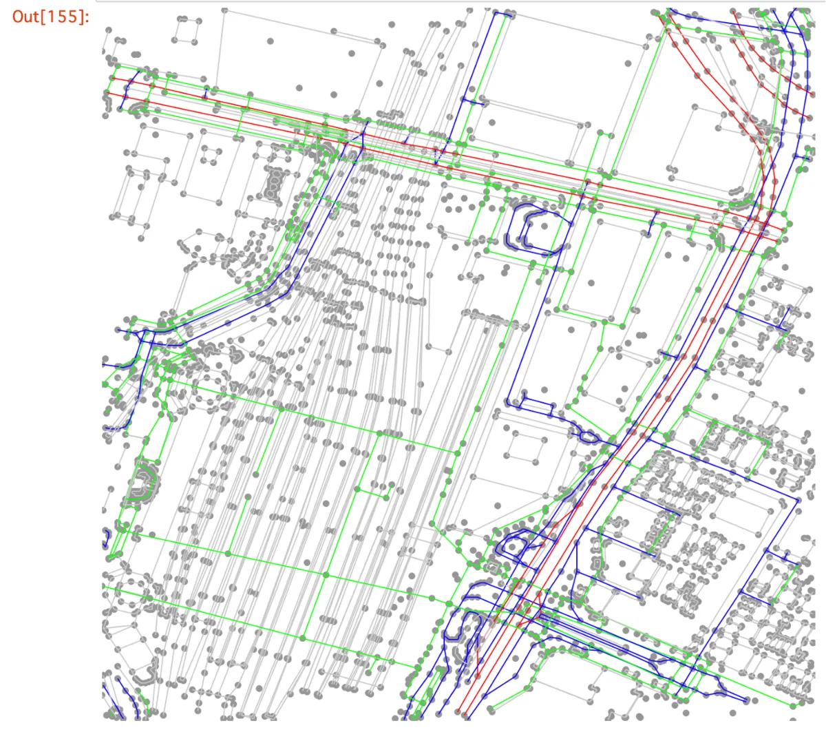
Here, Nodes are drawn as points using latitude and longitude coordinates, and Ways are drawn as colored lines by road type. Red lines are major roads, blue lines are general roads, green lines are pedestrian roads, and gray lines are other boundaries.

Conclusion

We set up an environment to run Rust in Jupyter Notebook, loaded OpenStreetMap data, and explored its structure. Rust runs fast, while still allowing relatively concise code for many kinds of data processing. Some parts feel unique at first, but they also encourage safer coding patterns. I hope this article serves as a useful starting point for trying more algorithms from here. For useful Rust libraries around OpenStreetMap, awesome-georust is a good reference.

Finally, NearMe is hiring engineers. This is a field with a lot of untapped potential, and we would love to hear from you if you are interested.

Apply here

Author: Kenji Hosoda