Introduction

In this article, we forecast ride demand for an advance-booking mobility service using time-series analysis. The key challenge is that there is a lag of several days between order time and ride time. In a typical setting, future demand is forecast only from historical demand fluctuations. For advance-booking services, however, it is reasonable to expect that already-booked future rides should improve the forecast.

Here, I generate toy data for advance bookings via simulation, build a time-series model that incorporates advance reservations, and evaluate it. I also provide a high-level summary of validation results on real data using the same modeling approach.

For time-series analysis, I used Darts, a Python library. It provides many forecasting models, including statistical methods and machine learning methods. It also offers a unified API for time-series operations, model training, and validation (reference). I will introduce it through code snippets as well. The full code used in this article is available here.

Creating Toy Data for Ride History

First, I randomly generate a list of ride timestamps so that their probability distribution has weekly, monthly, and quarterly periodicity.

from darts.utils.timeseries_generation import sine_timeseries, constant_timeseries
time_length = 365
sample_size = 10000
distribution = sum([
    sine_timeseries(length=time_length, value_frequency=(4/365), value_y_offset=1, freq='D'),
    sine_timeseries(length=time_length, value_frequency=(1/30), value_y_offset=1, freq='D'),
    sine_timeseries(length=time_length, value_frequency=(1/7), value_y_offset=1, freq='D'),
    constant_timeseries(length=time_length, value=1, freq='D')])
p_values = (distribution / distribution.sum()[0]).values()[:,0]
times = distribution.time_index.values
ride_start_dates = np.random.choice(times, size=sample_size, replace=True, p=p_values)

Then, I aggregate the data by day. The resulting time-series is stored as a TimeSeries.

from darts import TimeSeries
time_counts = dict(zip(times, np.zeros(times.shape)))
uniuqe, counts = np.unique(ride_start_dates, return_counts=True)
for time, value in zip(uniuqe, counts):
    time_counts[time] = value
target_series_df = pd.DataFrame(data=time_counts.items(), columns=['time', 'count'])
target_series = TimeSeries.from_dataframe(target_series_df, freq='D', time_col='time', value_cols='count')

Plotting it gives the following:

target_series.plot()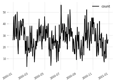

You can see the specified periodic patterns despite the noise.

Simple Forecasting

• Model setup

Here, I use Exponential Smoothing as a simple baseline time-series model. Internally, Darts uses the Holt-Winters method, which models trend and seasonality and combines smoothed components to estimate expected values (reference).

from darts.models import ExponentialSmoothing
model = ExponentialSmoothing()

• Training and forecasting

I split the data into training and test sets at a specific timestamp, train the model on the training data, and forecast the test period.

split_ts = pd.Timestamp('2000-11-01')
train, val = target_series.split_after(split_ts)
model.fit(train)
prediction = model.predict(len(val))

The following figure shows the result, plotting actual values (target) and predicted values (forecast).

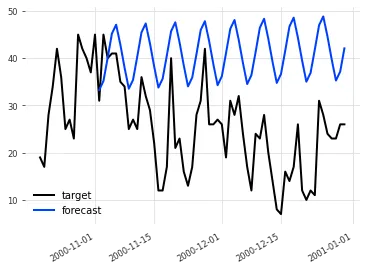
The forecast is relatively accurate at the beginning of the test period, but the error grows over time.

• Backtesting

To evaluate forecast accuracy quantitatively, I use backtesting. At each time step, the model is trained using data available up to that point and predicts values at a specified horizon.

backtest = model.historical_forecasts(
    series=target_series,
    forecast_horizon=forecast_horizon,
    start=split_ts - Timedelta(timedelta(days=forecast_horizon)))

Here, forecast_horizon specifies how many time steps ahead to forecast (days ahead in this case). start specifies when to begin forecasting. To align forecasted periods in backtesting, start is shifted by each forecast_horizon.

The next figure compares forecasts with horizons of 1 day and 10 days.

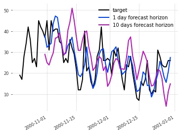
1 day forecast horizon is the one-day-ahead backtest forecast, and 10 days forecast horizon is the ten-day-ahead forecast. The one-day forecast fits the observed data better.

As an error metric between backtest forecasts and observed data, I use root mean squared error (RMSE). A smaller value indicates higher forecast accuracy.

from darts.metrics import rmse
print('Backtest RMSE = {}'.format(rmse(target_series, backtest)))

RMSE is 5.88 for a 1-day horizon and 10.75 for a 10-day horizon, indicating higher accuracy for the 1-day-ahead forecast.

• Comparison with a baseline model

To show that the previous model captures non-trivial time-series structure, I compare it with a simpler baseline model. Here, the baseline simply repeats the last observed training value for future predictions.

from darts.models import NaiveSeasonal
model = NaiveSeasonal(1)

The following figure plots RMSE by forecast horizon for both Exponential Smoothing and the baseline model.

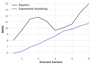
Exponential Smoothing has lower RMSE than the baseline for every horizon, meaning better accuracy throughout. Because the data has weekly periodicity, the baseline also improves around a 7-day horizon.

Creating Toy Data for Scheduled Rides

For each forecast horizon, I create data for rides already scheduled at that horizon.

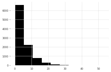
To do this, I first generate the gap between order time and ride time for each ride timestamp generated earlier. The gap follows an exponential distribution.

advanced_diffs = np.random.exponential(5, size=len(ride_start_dates))

Its histogram is shown below.

Then, I filter ride timestamps whose order-to-ride gap is at least the forecast horizon (plus aggregation timing), and count them by ride date.

def get_advanced_series(forecast_horizon):
    advanced_start_dates = ride_start_dates[np.where(advanced_diffs >=  forecast_horizon + 1)]
    time_counts = dict(zip(times, np.zeros(times.shape)))
    uniuqe, counts = np.unique(advanced_start_dates, return_counts=True)
    for time, value in zip(uniuqe, counts):
        time_counts[time] = value
    advanced_series_df = pd.DataFrame(data=time_counts.items(), columns=['time', 'count'])
    advanced_series = TimeSeries.from_dataframe(advanced_series_df, freq='D', time_col='time', value_cols='count')
    return advanced_series

The following figure plots scheduled rides for one day ahead (1 day advanced) and ten days ahead (10 days advanced) together with observed ride data.

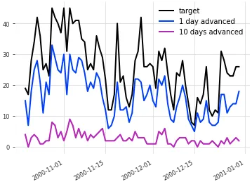
The one-day-ahead scheduled rides are naturally closer to observed data than the ten-day-ahead schedule. Still, even ten-day-ahead data contains useful signal.

Forecasting with Advance Reservations

• Model setup

This time, I use Linear Regression as a time-series model that incorporates advance reservations. It regresses the target observed value on multiple variables from both observed and scheduled-ride data. The model concept is shown below.

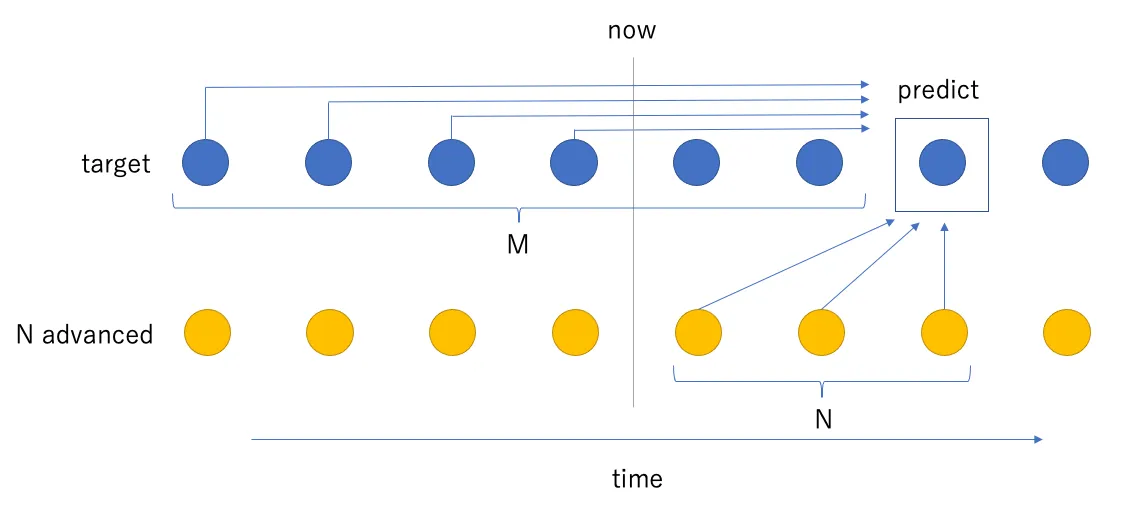
target is observed ride data, and N advanced is scheduled-ride data for N days ahead. To predict the observed value N days ahead, I use N future points of scheduled-ride data plus observed data from M points before the prediction point (predict) up to the current point (now). These features are collected along the time axis for training. A separate model is trained for each N.

In code, it looks like this:

from darts.models import RegressionModel
model_N = RegressionModel(lags=list(range(-M, 1 - N)), lags_future_covariates=list(range(1 - N, 1)) )

lags specifies the window of observed data used for training relative to the prediction point. lags_future_covariates specifies the window of scheduled data used for training. future_covariates represents known future information, such as weather forecasts (reference).

• Model evaluation

I evaluate this model with backtesting as well.

backtest = model_N.historical_forecasts(
    series=target_series,
    future_covariates=get_advanced_series(N),
    forecast_horizon=1,
    start=split_ts - Timedelta(timedelta(days=1))

Here, N-days-ahead scheduled-ride data is provided as future_covariates. Since the model is indexed around the prediction point, forecast_horizon is set to 1.

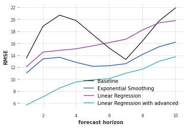
Next, I plot RMSE against forecast horizon. I also include results from other models for comparison.

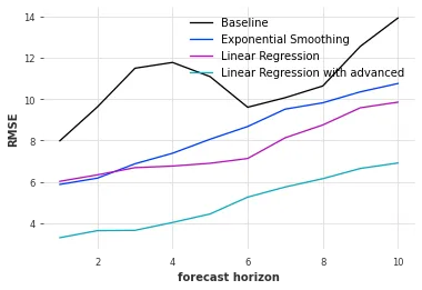
Linear Regression with advanced is the linear model with advance reservations. Linear Regression is the same model without future_covariates. Exponential Smoothing and Baseline are the models introduced earlier. The linear model with advance reservations achieves the lowest RMSE, and thus the best accuracy, across all forecast horizons.

• Evaluation on real data

Finally, I applied the same analysis to real order data extracted under specific conditions. I omit the exact details, but the real data distribution is reasonably similar to the toy data above.

As shown in the figure, the linear regression model that incorporates advance reservations also achieved the highest forecast accuracy on real data, consistent with the toy-data results.

Other Models

In the published code, in addition to linear regression, I also tested LightGBM, a nonlinear gradient boosting approach. In this dataset, linear regression performed slightly better. A likely reason is that local temporal relationships are strongly linear.

I also built and evaluated models that include day-of-week information encoded with sine/cosine features. Including weekday information slightly improved accuracy, especially for horizons longer than one week. This suggests that explicit periodic signals help forecasting.

Darts also offers many neural-network-based models, but I excluded them from this article’s scope. They require more computation and careful hyperparameter tuning, and they are generally better suited to larger and more complex datasets.

Conclusion

I applied time-series analysis to advance-booking ride-order data and showed that models incorporating advance reservation information can forecast ride demand more accurately. I also showed that Darts makes this type of analysis relatively easy to implement. Predicting the future from historical data is important in many parts of service development, and I hope this analysis serves as a useful starting point.

Finally, NearMe is hiring engineers. There is still a lot of untapped potential in this domain, so if you are interested, please apply using the link below.

• Careers page

Author: Kenji Hosoda